How does ILEX work?

ILEX is primarily a toolkit for analysing High time resolution (HTR) Fast Radio Burst (FRB) data produced by the CRAFT Effortless and Localisation and Enhanced Burst Inspection (CELEBI) pipeline.

CELEBI paper - https://www.sciencedirect.com/science/article/abs/pii/S2213133723000392 CELEBI github - https://github.com/askap-craco/CELEBI

However, fundamentally, ILEX will work with Stokes I, Q, U and V frequency and time dynamic spectra regardless of context.

Currently, ILEX only supports 2D numpy files .npy.

The `FRB` class

The main class that you will be using is the FRB class. This class can be imported by running

from ilex.frb import FRB

This class has a variety of functions that can be used to plot, fit and manipulate Stokes data. Currently the FRB class supports:

manipulating data: including cropping, channel zapping
processing data: including averaging, weighting, Faraday de-rotating, normalising
Fitting the time series to a sum of Gaussian pulses convolved with a one-sided exponential tail
Deriving a decorrelation bandwidth
Fitting the Rotation Measure (RM) using either Q/U fitting or RM synthesis
Plotting data: including time series, frequency spectra, dynamic spectra, PA, poincare sphere

Initialising the `FRB` class

Create a new instance of the FRB class. Here we can specify a number of parameters, I recommend at the very least setting cfreq and name. Here we set cfreq, the central frequency, to 919.5 MHz

frb = FRB(name = "FRBtest", cfreq = 919.5)

We can also initialise the class using a config file,

frb = FRB(yaml_file = "config.yaml")

see the tutorial on FRB config files for more details Tutorial 3: ILEX config files.

To start using the FRB class, we need to load in data, there are 4 data products that can be loaded in, dsI, dsQ, dsU and dsV, these represent the Stokes I, Q, U and V dynamic spectum.

# loading in Stokes I dynamic spectrum
frb.load_data(dsI = "dsI.npy")

The `FRB` parameters

The parameters in the FRB class are split into 3 groups (for the most part…)

par      - parameters that are descriptive to the FRB data, such as name, intrinsic data resolution etc.
metapar  - meta parameters that describe the processing being done on the FRB data, such as time,freq crops, averaging etc.
hyperpar - hyper parameters that describe the functionality of the class itself, such as if verbose printing, showing plots etc.

frb.par is where you can find all the parameters of the FRB.

frb.metapar is where you can find all the meta parameters of the FRB.

Each hyper parameter is their own attribute in the FRB class, such as verbose, i.e. frb.verbose or show_plots, frb.show_plots

`par`

There are a number of parameters that can be set that for the most part are only descriptive of the FRB, these include

name        - The name of the FRB, this is used when saving plots as .png files
RA          - Right Ascension of FRB position (Metadata)
DEC         - Declination of FRB position (Metadata)
DM          - Dispersion Measure (Metadata)
bw          - Bandwidth of FRB observation
MJD         - Modified Julian Date [days] of burst (Metadata)
cfreq       - Central frequency [MHz] of bandwidth
t_lim_base  - Base limits of loaded FRB data in time [ms]
f_lim_base  - Base limits of loaded FRB data in freq [MHz]
t_ref       - Zero-point of data in time [ms], i.e. reference point
nchan       - Number of channels in Dynamic spectra
nsamp       - Number of time samples in Dynamic spectra
dt          - Intrinsic resolution of time samples in loaded Dynamic spectra
df          - Intrinsic resolution of freq channels in loaded Dynamic spectra
RM          - Rotation Measure
f0          - Reference frequency [MHz]
pa0         - Reference Polarisation Position Angle (PA)
tW          - Weights applied in time when averaging to make spectra
fW          - Weights applied in frequency when averaging to make time series

Note: Parameters labelled with (Metadata) are purely descriptive labels that are not used any where in ILEX (yet…).

`metapar`

These meta parameter control the processing of the FRB data, this includes

t_crop      - Crop of on-pulse data in time [ms] or in phase units
f_crop      - Crop of on-pulse/off-pulse data in frequency [MHz] or in phase units
terr_crop   - Crop of off-pulse data in time [ms] or in phase units. Used to estimate time and freq noise/errors
tN          - Averaging factor in time
fN          - Averaging factor in frequency
norm        - Normalisation
zapchan     - Channel zapping

`hyperpar`

These hyper parameters control many of the class utilities. This includes

verbose     - Enable verbose printing, this will enable the logging features of ILEX
plot_type   - Type of plot when plotting 1D data, [lines] for line plots and [scatter] for scatter plots
residuals   - If true, plots of fitting results will also show residuals
apply_tW    - If true, will apply time weights [tW]
apply_fW    - If true, will apply freq weights [fW]
zap         - If true, the FRB data will be treated as if channels are zapped and will use numpy .nan functions when processing
show_plots  - If true, show any plot in an interactive window
save_plots  - If true, save any plot as a .png file
crop_units  - Control what units are used when cropping data, [physical] for ms/MHz or [phase] for phase units [0.0 - 1.0]

All the above par, metapar and hyperpar parameters can be set in a config file for ease of use and reproducibility.

How data is processed in the `FRB` class

ILEX by default will not load in the Stokes dynamic spectra files into memory all at once, they will be loaded in as memory maps to the files on disk (see https://numpy.org/doc/stable/reference/generated/numpy.memmap.html). Every time the user requests some data, whether for plotting, fitting etc., ILEX will first define a “crop”. This crop has two main parameters, t_crop and f_crop, these define the crop boundary in time [ms] and frequency [MHz] by default. ILEX will then take this crop, and load in the data within this crop into memory. This makes ILEX extremely memory efficient and in most cases quick as well, since that data will be cached when being used again. The image below illustrates this.

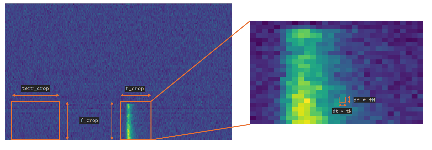
This crop is also refered to as the on-pulse crop, as such we try to capture the FRB within this crop. In addition to this crop, we can also specify an off-pulse crop that will use off-pulse data to estimate the noise per time sample per frequency bin. This off-pulse crop uses the same f_crop parameter to crop in frequency and to specify the off-pulse crop in time we can use terr_crop.

Once the crop boundaries are defined, ILEX will process the data. Currently ILEX supports the following processing techniques:

Averaging

We can average the data in both time in frequency, i.e. downsample by some factor. For example, if we want to downsample 1us data to 10us data, we can do this by specifying tN = 10, same with frequency but using fN.

Channel zapping

We can zap any channels if there is bad RFI etc. We can do this by specifying zapchan. For example, if we set zapchan = "1100:1150", all the channels between 1100 MHz and 1150 MHz (inclusive) will be zapped and ignored during processing. We can specify as many regions of frequency as we want, for example zapchan = 1100:1150, 1180:1220 will now also zap the channels between 1180 MHz and 1220 MHz. We can also specify singular channels, zapchan = 1100:1150, 1160, this will also zap the channel at 1160 MHz.

NOTE: depending on df * fN this may not be perfectly precise.

Faraday de-rotating

We can de-faraday rotate the Stokes Q and U data by specifying RM and f0. If f0 is not set, then it will take the default value of f0 = cfreq, i.e. the central frequency.

Weighting

We can weight in time and frequency. When we specify time and frequency weights tW and fW, these will only be applied when we are averaging the entire crop. For example, if we are making frequency spectra, we average over all the time bins, in this case the time weights tW will be applied. Same case for the frequency weights fW.

We can set the weights using

# setting frequency weights
frb.set_weights(xtype = "t")

where xtype = "t" or "f" denotes if we are setting the time or frequency weights.

The following is a list of the types of weights we can apply.

Define a list of weights to apply

We can set a list of weights

frb.set_weights(xtype = "t", W = [1, 2, 3, 4,...])

just make sure the number of weights matches the number of time samples in your crop. You can also just define a single scalar value, although this is less useful.

frb.set_weights(xtype = "t", W = 2)

interpolation

We can define a set of weights along with x values that can be used to interpolate between these weights, for example

# 1000 weights from 0 to 1
W = np.linspace(0, 1.0, 1000)

# x coordinate for weights
x = np.linspace(1, 1000, 1000)

# set weights, make sure to use interp method
frb.par.set_weights(xtype = "t", W = W, x = x, method = "interp")

# define a new set of x coordinate somewhere inbetween 1 and 1000
x_int = np.linspace(401, 500, 100)

# interpolate weights
W_int = frb.par.tW.get_weights(x = x_int)

This is useful to define a set of weights for the full extent of an FRB or the dataset, this interpolation will then work with your crop.

Define a weight function

We can also define a function that will when evaluated will produce weights that will be applied directly to the data. This allows us to be creative. See the advanced ILEX Tutorial for an example Tutorial 2: Fitting methods.

NOTE: Weights are applied after averaging in time or frequency using tN or fN.

normalising

We can also normalise the data if desired, although this hasn’t been tested, so use at your own discretion. (This may be removed in a later version of ILEX, so probably don’t rely on it too much)

norm = max - normalise using maximum max() norm = absmax - normalise using absolute maximum abs(max()) norm = None - Skip normalisation (default)

Order of process operations

The order in which data is processed goes like this:

Crop in Time
Crop in freq
Channel zapping
normalise (may be removed)
Faraday de-rotate
Time average
Freq average
Time weights
Freq weights
Produce data products, including noise/error products

The Data products

The .get_data() is the most important function in the FRB class as this is what retrieves the full processed Stokes data products. The following data products can be called:

dsI, tI or fI - For the Stokes \(I\) dynamic spectrum, time profile and frequency spectrum
dsQ, tQ or fQ - For the Stokes \(Q\) dynamic spectrum, time profile and frequency spectrum
dsU, tU or fU - For the Stokes \(U\) dynamic spectrum, time profile and frequency spectrum
dsV, tV or fV - For the Stokes \(V\) dynamic spectrum, time profile and frequency spectrum
tL or fL - For the Stokes \(L\) time profile and frequency spectrum
tL or fL - For the Stokes \(P\) time profile and frequency spectrum.

data = frb.get_data(["dsI", "dsQ"], get = True)

This call to .get_data() is requesting a crop of the stokes I and Q dynamic spectra. This will run through all the processing steps outlined above and spit out cropped and processed stokes I and Q dynamic spectra, denoted by the ds. We also return these data products as a dict by specifying get = True.

We can also ask for 1D time series data and/or spectra data

data = frb.get_data(["dsI", "dsQ", "tI", "fI"], get = True)

here we have also asked for the Stokes I 1D times series (denoted by the t) and frequency spectra (denoted by the f). When we ask for any 1D data products, if we have also defined the off-pulse crop using terr_crop, the .get_data() method will also return the corresponding noise/error products with the suffix err, in this case tIerr and fIerr. Additionally, the x-axis for the times series time and frequency spectra freq will also be saved.

Any data product that is created will always be saved to the FRB class, for example

"dsI", "dsQ" will be saved to FRB._ds, if you want to retrieve "dsI", you specify FRB._ds["I"].

Similarly with time series, FRB._t and frequency spectra FRB._f. In the case that you also want the noise/error data as well, specify FRB._t["{S}err"] for any Stokes parameter S in the case for time series noise (Same thing for frequency spectra). For the time series/freq spectra x-axis, specify FRB._time/FRB._freq.

You can also ask for the fractional Stokes parameters (i.e. \(Q/I\) etc.). To do this set ratio = True

data = frb.get_data(["tQ", "tU"], get = True, ratio = True)

You can only ask for the fractional Stokes parameters for Stokes \(Q, U, V, L\) and \(P\). Additionally you can only ask for their respective time profiles and/or frequency profiles (t or f). If, for example you ask for an additional Stokes product that doesn’t support ratio, the function will just return the default paramter

data = frb.get_data(["dsI", "tQ"], get = True, ratio = True)

In this case, dsI will be the original stokes \(I\) dynamic spectrum, whilst tQ will be the time profile of \(Q/I\).

Stokes \(L\) and \(P\)

When using .get_data() to retrieve Stokes \(L\) and \(P\) products, it is useful to debias them. This can be done by setting debias = True

data = frb.get_data("tL", get = True, debias = True).

data instances

Every time .get_data() is run, an instance of the frb.par and frb.metapar attributes are created and labelled frb.this_par and frb.this_metapar respectivley. These parameters describe the processed data at that very instance. These parameters may differ from the base parameters set in the FRB class depending on if any of the par or metapar parameters were overwritten when calling an FRB class method, for example

frb.get_data(["dsI", "dsQ"], tN = 20)

in this example we have overwritten the tN parameter to 20. Thus if frb.this_metapar.tN will be 20 whilst the base value frb.metapar.tN will remain the same. This allows the user to quickly change any FRB/crop parameters to explore the data without having to update a config file or the FRB class itself every time.

You can also change the hyperpar parameters (such as verbose), but these will be permanently changed.

NOTE: you can also change any of these parameters permanently using FRB.set().