Tutorial 1: Loading and plotting data
This brief tutorial will go through an example of using ILEX. The example data being used is an ASKAP observation of the FRB 20220610A, details of the FRB can be found in the following paper:
https://www.science.org/doi/abs/10.1126/science.adf2678
Loading data
We will start by importing the ilex FRB class, this class holds all the useful functions we will need to study this FRB.
from ilex.frb import FRB
import matplotlib.pyplot as plt     # for external plotting
Then we will load in our FRB data. Example data can be found in examples/. For now we will load in
the Stokes Power dynamic spectrum, i.e. dsI
frb = FRB(name = "FRB220610", cfreq = 1271.5, bw = 336, dt = 50e-3, df = 4)
frb.load_data(dsI = "examples/220610_dsI.npy")
In the above code, we initialised an instance of the FRB class and named the instance FRB220610. FRB220610 has a
central frequency and bandwidth of 1271.5 MHz and 336 MHz respectively, hence we set cfreq = 1271.5 and
bw = 336. The data we are loading in has an intrinsic time and frequency resolution of 50 us and 4 MHz respectively,
so we also need to set dt = 0.050 and df = 4. It is important to note that time and frequency are in units of milliseconds (ms)
and MHz respectively.
Cropping and plotting data
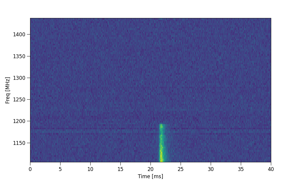
Now that the data is loaded in, we want to plot it. We can do so by simply calling the .plot_data() method.
Here we are going to plot the full Stokes I dynamic spectrum. Make sure to set either show_plots or save_plots
to True (show_plots enables interactive windows, save_plots saves png files of the plots)
frb.plot_data("dsI", show_plots = True)
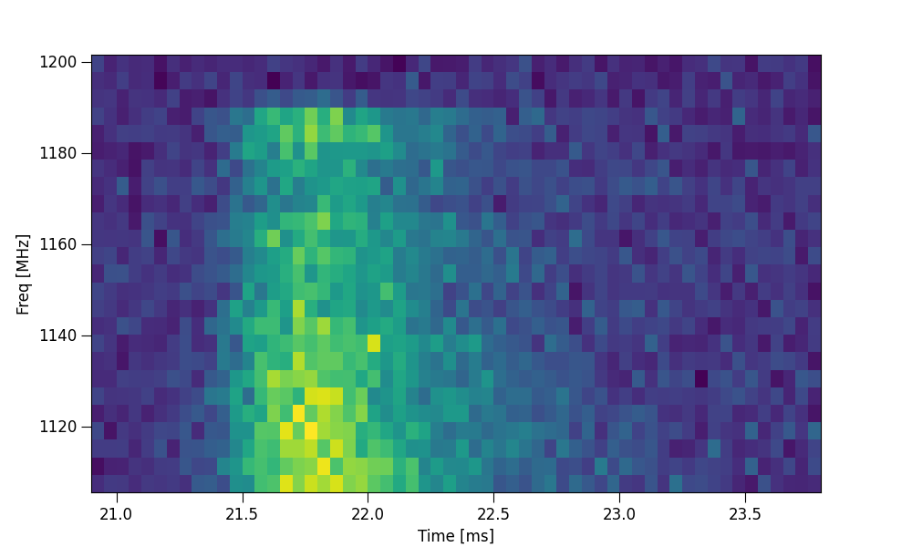
Everytime ILEX uses data for plotting, fitting etc. a crop is used, since FRBs are very narrow. To define a crop the t_crop
and f_crop parameters must be specified. By default they are ["min", "max"] which denotes the entire
dynamic spectrum.
frb.plot_data("dsI", t_crop = [20.9, 23.8], f_crop = [1103.5, 1200])
There are various other plotting functions that ILEX provides, however, for 99% of cases a user may want to create there own plots. In which case, ILEX can act more like a data container to retrieve processed data for plotting.
processing data and the get_data() function
Perhaps the most powerful class method in ILEX is the .get_data() method.
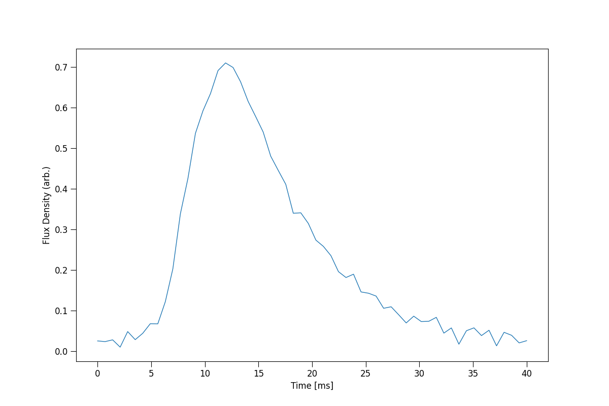
As a simple excersise we will retrieve a crop of the above FRB and plot the stokes I time series profile.
# get time series profile
frb.set(t_crop = [20.9, 23.8], f_crop = [1103.5, 1200])     # set crop params, can also just pass these in the .get_data() method
tI = frb.get_data(data_list = ["tI"], get = True)['tI']     # get data

# make x axis array
x = np.linspace(*frb.par.t_lim, tI.size)

# plot
plt.figure(figsize = (12,8))
plt.plot(x, tI)
plt.xlabel("Time [ms]")
plt.ylabel("Flux Density (arb.)")
plt.show()
Saving data
Data crops can be saved to file. Note: you do not need to call the .get_data() method since this will be done when
.save_data() is called.
frb.save_data(data_list = ['tI'])
This will save a .npy file called FRB220610_tI.npy. Multiple files will be saved depending on the list of data products
provided to the .get_data() method.